the proximitor

This article describes how the displacement sensor works or proximitor, often used in turbomachinery oil film bearings. This analysis is usually performed with vibration monitors.

These sensors are also called relative vibration sensors..

In turbomachinery this type of bearings are normally instrumented with displacement sensors. (proximitors).

De facto, with proximitors, its degradation, or malfunction, can be better monitored and inserted in a program of Predictive maintenance.

2 – Constitution of the proximitor measurement system

A complete proximity probe system consists of:

• a probe,
• extension cord
• driver

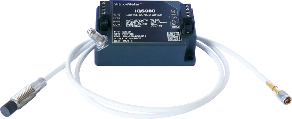
Figure 2 – Creation of a displacement measurement system with proximitor. The sensor+ the extension cable + the conditioner (driver)

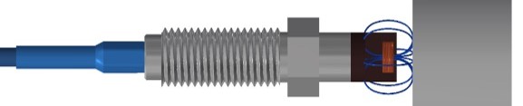
The working principle of proximitors is as follows:

• As the shaft moves across the surface of the probe, the magnetic field is absorbed by the surface of the material
• Eddy currents are formed in the shaft material, attenuating the probe coil field.
• As a result, changing the range of the DC voltage then converts that value into a signal of 200 mV / mil AC. (for example; depends on the sensitivity of the probe)

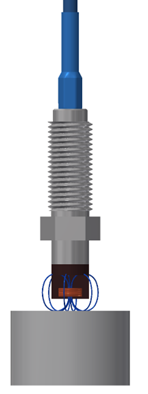
Figure 4 – Working principle of a proximitor

This means that the shaft material in front of the probe generates changes in the probe's electromagnetic field that are used to measure the distance between the shaft tip and the shaft..

Below you can see a video with an introduction to proximitors.

3 Output voltage of a proximitor driver

In the figure below, you can see the voltage measured at the driver output as a function of distance.

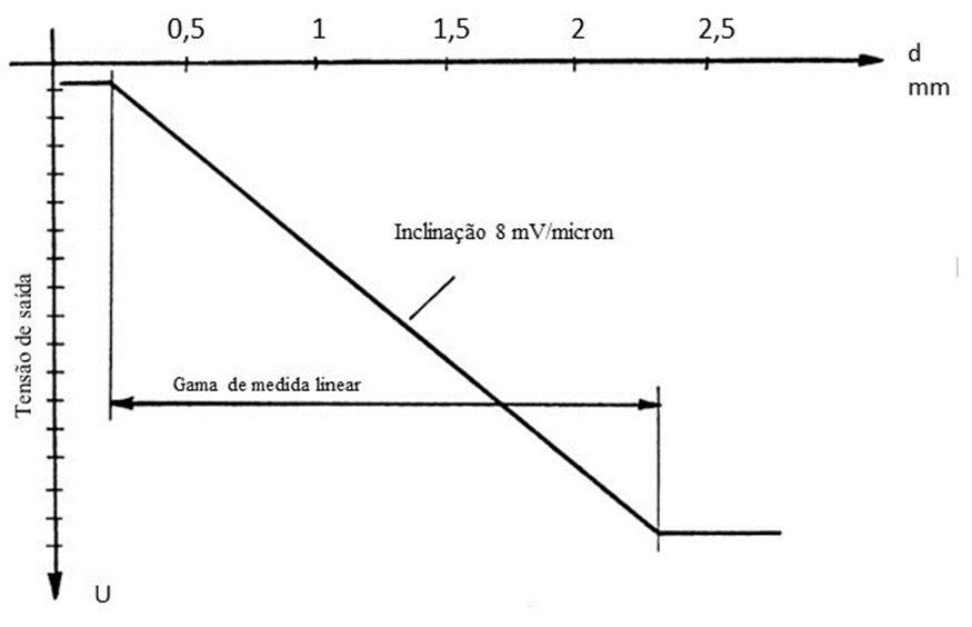
Figure 4 – Output voltage of a proximitor driver

The greater the distance between the probe tip and the shaft, the smaller the voltage. It should be noted that these sensors are powered by a power supply. -24 VDC.

When the shaft starts to rotate, two signals are measured at the driver output:

• A DC signal proportional to the average distance from the sensor tip to the shaft, also known as DC-GAP
• An AC signal proportional to vibration.

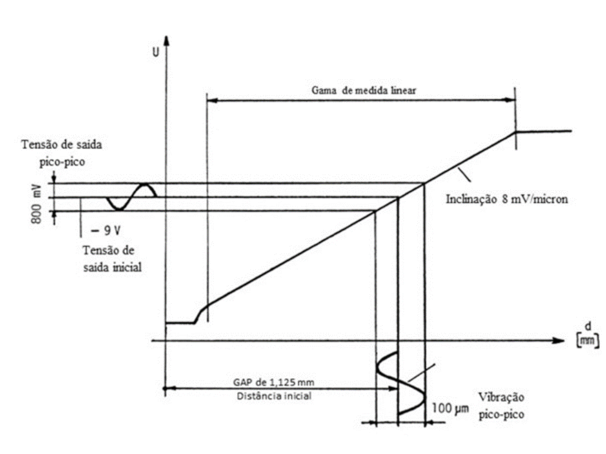
Figure 5 – Signal at the driver output when the shaft rotates

Below you can see a video about measurements with proximitors.

Below you can see a video about the proximitors GAP.

4 The linear measurement range of the proximitor

In the previous figures the linear measurement range is marked, which corresponds to the range of distances between the probe tip and the shaft, where the measurement is correct.

In the technical specification of a proximitor you can see the following graph.

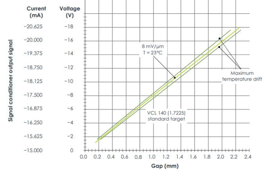
Figure 6 – Output of the signal conditioner of a Vibrometer ISQ900 proximitor

It can be seen from this graph that the linear measurement range lies between about -2 e -18 VDC and corresponds to a range of 2 mm away.

In the same specification one can read:

Linear measuring range (typical):

0,2 a 2,2 mm, corresponding to an output of -1,6 a -17,6 V

5 The sensitivity of the proximitor

There are proximitors with different sensitivities, for example:

• 8 mv /micron common in steam turbines and linear measurement range of 2 mm
• 4 mv/micron common in hydro generating sets and linear measurement range of 4 mm

6 Assembling a proximitor and checking it

The proximitor must be mounted so that the distance from the sensor tip to the shaft is in the middle of its linear range.

In the previous case the middle of its linear range is:

Align range =-17.6- (-1,6)= -16 V

Middle of linear range= -8 V

Like this, in this case, the DC output signal from the sensor, after assembled, with the machine stopped, is – 8V.

This needs to be checked, with the machine stopped, after sensor assembly is carried out.

In the figure below you can see the configuration of a proximity sensor in a Vibrometer permanent monitoring system..

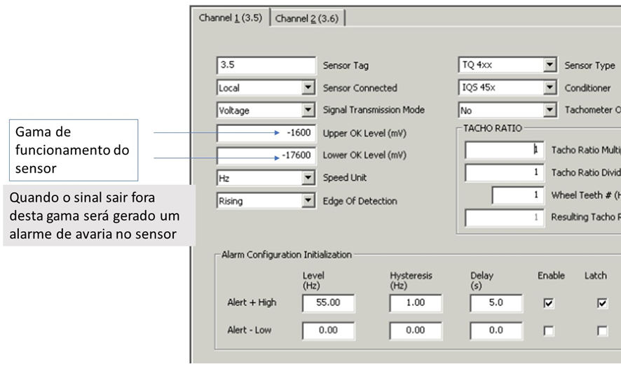
Figure 7 – Configuring a proximity sensor in the Vibrometer MPS1 program

7 -Verification of the proximitor assembly in a permanent monitoring system

In the photograph shown below, you can see readings of the distance from the tip of two proximity sensors to the shaft, with a generator set stopped, MPS2 program for Vibrometer.

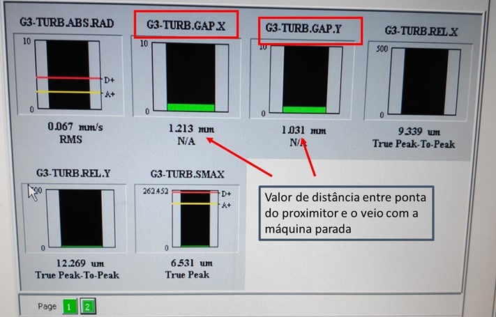
Figure 8 – In the photograph where you can see readings of the distance from the tip of two proximity sensors to the shaft, with a generator set stopped, MPS2 program for Vibrometer.

This screen directly displays the distances because their sensitivity in mV/micron was introduced when configuring the sensors..

To know if these probes are properly mounted, you must know the linear range of the proximity sensors mounted there.:

• If they have a linear range of 2 mm are more or less, one is fine and the other is more or less.
• If they have a linear range of 4 mm, they are both poorly assembled because they are very far from the midpoint of the linear range, which is from 2 mm.

8 – Irregularities in the shaft – O run-out

From the above it is understood that these probes function as contactless comparators. Measure the relative distance between the probe tip and the shaft. Hence they are also designated, often, relative vibration sensors.

So you have to, if there are irregularities on the surface of the shaft, these will be measured and mixed with the vibrations. These irregularities are called run-out.

There are two types of run-out:

• The mechanic;
• the electric.

Causes of mechanical runout:

• Improper milling of spindles (egg shape).
• Worn rotor (thermal or mechanical).
• surface irregularities – scratches, bumps, imperfections.

Causes of electrical runout:

• localized magnetism.
• Alloys on the metal shaft are not evenly distributed (low quality material).
• Residual stress concentration.

The probe measures total runout = mechanical + electric

Care must be taken to prepare the target area of ​​the shaft and protect it.

On analysis vibrações of the displacement waveform (in microns) measured with a proximitor, then presented, made with a vibration analyzer, you can see the effect of runout on the wave and its spectrum.

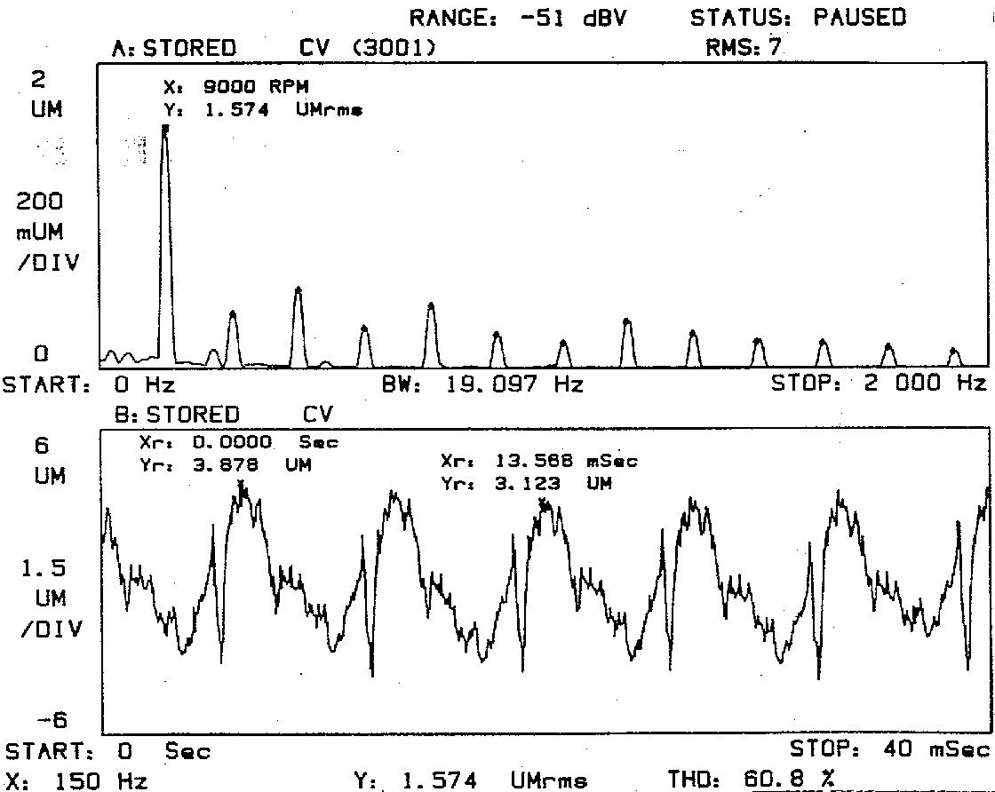
In the wave you can see the effect of a scratch on the shaft, and in the spectrum one can see the numerous harmonics generated by the existence of this risk.

In the figure below, you can see a shaft with a, which geometrically is circular, but whose base material is ovalized.

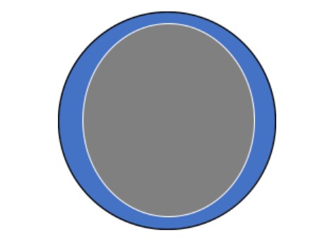
This ovalization will cause a runout with waveform effects, across spectrum and global levels.

9 The frequency response of the proximitor

The operating frequency of these sensors is typically between Hz and 20 KHZ.

10 Pros and cons of proximitors

The advantages and disadvantages of proximitors are as follows:

Benefits:

• no contact.
• Measures relative shaft vibration.
• Measures axis centerline position (DC clearance).
• Measure the axial position (impulse).
• DC Flat Frequency Response – 20KHz.
• simple calibration.
• Suitable for harsh environments.

Disadvantages:

• The probe can move (vibrate);
• Does not work on all metals;
• Coated shafts will provide false measurements;
• Measurement is affected by scratches and tool marks on shaft (runout)

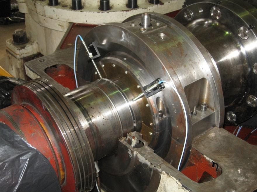
11 Vibration analysis with proximitors in machines with oil film bearings

The time signal provides important and useful information, but as the shaft moves along a two-dimensional path, this information is limited. In this type of movement, on anti-friction metal bearings, where the oil film dampens vibrations in the bearing housing, the signal in time, supplied by an accelerometer, is not the most suitable.

To monitor this movement, displacement sensors that measure the relative vibration between the shaft and the housing, are more suitable, especially when installed in pairs.

With two relative vibration displacement sensors (proximitors) there are conditions to know the movement of the center of the shaft in this plane.

This information can be presented in two individual time signals, respectively to each sensor, more or ideal, is to obtain a graph that represents the two dimensions of the movement of the shaft. This graph is designated by orbit.

The orbit represents the path from the center of the shaft in the reading plane of the pair of proximity sensors.

The sensors are rigidly mounted on the machine frame, next to the support areas of the shaft (bearings). Like this, the orbit represents the trajectory of the center of the shaft relative to the structure of the machine.

Due to the easy interpretation and amount of information that the graph contains, the hourglass, reconciled with a phase indicator, also known as a phase sensor, is an effective graph to understand the physical phenomena that occur on rotating machines.

12 – Orbit Construction

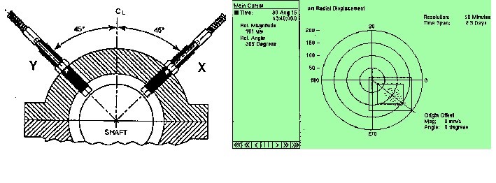
 The orbit combines the data present in the waveforms of the pair of proximity sensors, out of phase 90º, to create a graph that displays the movement of the shaft center in two dimensions. In the orbit of the Figure 13 the sensors are set at 0 ° and 90 °.

In orbit, a point is defined by a pair of X and Y values, obtained through the information contained in the signals in time.

The center of the graph is defined by the average of X values ​​and Y values ​​of the two waveforms.

An impulse emitted by phase sensor acts as a reference: the black dot shows the location of the center of the shaft when this impulse occurs.

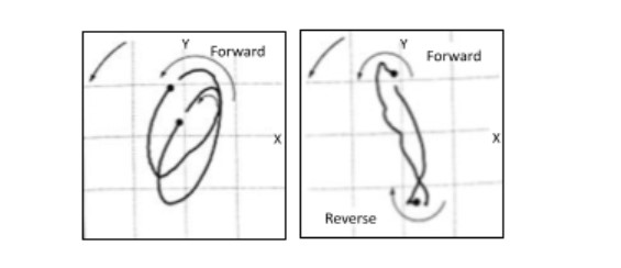
To complete the graph, the location of the sensors and the direction of rotation of the shaft are shown in Figure.13.

Note that the direction of rotation of the shaft cannot be determined from the orbit without additional information. The best way to determine the direction of rotation is to examine the machine. Another option is to use orbits in slow rotation, which act in the direction of the precession movement.

Like this, knowing that the machine is in slow rotation, allows to determine the direction of rotation observing the direction of precession. 

The direction of precession is determined by the space / black point sequence of the orbit of Figure 13. The point of maximum amplitude of the time signals corresponds to the minimum distance between the sensor and the shaft surface.

In the figure 13 illustrates the progression of the shaft center around its orbit from the point 1 to the 5. The point 1 shows the location of the center of the shaft when the pulse of the phase sensor, that is, when the first vertex of the notch produced in the shaft passes along the phase sensor. The dots 2 e 4 refer to the furthest and closest point to the X sensor (the minimum and maximum peak in the signal graph at time X). In the same way, The dots 3 e 5 refer to the furthest and closest point to the Y sensor (the minimum and maximum peak in the signal graph at time Y).

Usually, various vibration cycles are represented on the graph. In the figure 13, a vibration cycle is represented in the signal graph over time, which means that the orbit also has a cycle. The positive peak of the signal over time always represents the closest approximation of the shaft to the associated sensor.

13 – Mounting orientation of the sensors

The mounting directions for the sensors are defined in relation to the reference direction of the machine.

The observer will be positioned in the axial direction of the shaft from the driving machine to the driven machine.

The locations of the sensors are indicated at the ends of the graphs, which provides a uniform visual reference, regardless of the mounting orientation of the sensors. In the figure 14, The orbit is oriented so that, whoever watches her, view as being positioned according to the reference direction, looking along the axis of the machine.

Figure A 14 shows two examples of orbits with different orientations in the assembly of the sensors. In both cases, the orbit is the same, only the mounting orientation is different. Note that the indication of the sensors in the graphs represents the mounting position of these.

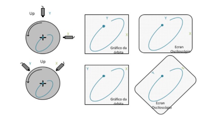
On the right side of the Figure 14, equivalent orbits from an oscilloscope are present. Because the X and Y axes of the bottom oscilloscope do not correspond to the positions of the mounted sensors, the oscilloscope would have to be physically rotated 45 °, counterclockwise (How does it happen?), in order to display the orbit with the correct orientation. In this orientation, the oscilloscope's horizontal and vertical axes match the sensor orientations.

When observing orbits on an oscilloscope, the X and Y axes of this, must comply with the installation instructions for the sensors, or the displayed orbit will not correspond to reality.

The filtered orbits are not built directly from the information indicated by the waveform pair. The time signal collected by the sensors is filtered at a certain frequency and later used for the construction of the filtered orbit.

14 – The phase and rotational speed reference – Phase sensor (keyphasor)

The space / orbit point sequence represents the effect of the phase sensor. This impulse represents an event in time that occurs once per rotation of the shaft. The signal comes from a particular proximity sensor that is placed radially in a different axial position.

The impulse of the phase sensor allows you to indicate the location of the center of the shaft at the moment when, the notch produced on the shaft for the purpose, go through this sensor during rotation. The space / point sequence indicates the direction of time increment.

Figure A 15 displays a rotating shaft. During the rotation movement, the center of the shaft also moves (precession movement) along a trajectory that will define the orbit. When the first vertex of the notch passes near the phase sensor (position 3 from Figure 15), the center of the shaft coincides with the phase sensor point of the orbit.

At the sign in time, the period between two impulses of the phase sensor represents a rotation of the shaft. In the orbit graph, the shaft moves along the path between two points of the phase sensor, during rotation. The point of phase sensor is added to the graph each time the shaft completes a rotation. If the graph covers information for multiple rotations, will be present, on this graph, the corresponding number of points phase sensor. 

In filtered orbits the nX the rotation speed, in which n it is an integer, successive points will be inserted in the graph phase sensor, that will overlap each other. The point of phase sensor adds information that is useful for determining the instantaneous direction of movement of the shaft and for estimating the absolute phase, the frequency of vibration in orders of the speed of rotation and, by last, the rotor vibration mode.

15 – the proximitor – iinformation present in the Orbits

The clock, especially be endowed with phase sensor, can be used to measure peak-to-peak amplitude in any radial direction, the relative frequency of the vibration or the direction of precession.

The orbit profile can provide important clues about the machines' behavior, highlight changes in the response that would have been traditionally unnoticeable, and help identify the location where the problem may occur in relation to the position of the machine components. The orbit displays the path of the shaft relative to the average position, there is no information about the average position of the shaft. To obtain the average position of the shaft, there are other types of graphics.

Orbit charts can be created from the same location and at different speeds (transient data), to show the evolution of shaft vibration with increasing speed. On the other hand, orbits can be created from different axial locations and at the same speed, to display the shaft vibration mode.

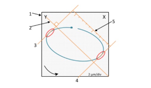
The main measurement that can be made in an orbit is the peak-to-peak amplitude (Figure 16). 

There are two fundamental aspects when using this measurement.

• First, peak-to-peak measurement needs to be done parallel to the sensor's measurement axis. Simply measure vertically or horizontally, in this case, would produce different and incorrect results.
• Second, peak-to-peak measurement is made between tangents that are also perpendicular to the sensor's measurement axis.

The orbit is used to determine the direction of shaft precession.

The point of phase sensor indicates the direction of time increase, sense that will be the precession of the vein. Once determined, the direction of precession can be compared to the direction of rotation to confirm that we are facing precession to face (coinciding direction of rotation and precession) or back (sense of precession contrary to rotation).

In complex orbits, the shaft may undergo forward precession during one part and backward precession during the remainder of the orbit profile.

Notice how the inner loops of the orbits 1 / 2X the rotation speed of the Figure 17 keep precession forward, while outer loops show backward precession.

The filtered orbit can be used to estimate the absolute phase of the two components of the signal.

This estimate will be more accurate for circular orbits, and less accurate for elliptical orbits (Figure 18) due to the constant angular velocity of the circular orbit along its path (equal time intervals and similar angles between points). 

In elliptical orbits, the angular velocity of the orbit is not constant (equal time intervals, but different angles between points). Since the phase is a measure of time, these variations in angular velocity cause inaccuracies when trying to estimate the phase with respect to each sensor.

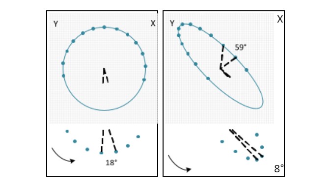
Figure A 19 illustrates a set of orbits 1X the speed of rotation at which the points of the phase sensor indicate the location of the center of the shaft, in each measurement plan, the moment the impulse occurs. These points can be connected to each other by a line, in order to obtain an estimate of the behavior of the shaft along its length.

The shaft movement occurs at different rates in different parts of the orbit. No additional indications, the location of the shaft is not known at any given time.

The impulse of the phase sensor is the solution, providing the reference in time for a point, in particular, in each orbit.

16 – the proximitor – Orbit presentation associated with the signal waveforms in time

This type of graph combines the orbit with two waveforms of the signal in time. The waveform resulting from the Y reading is displayed above the X, both to the right of the orbit (Figure 20).

The graph contains information about the direction of rotation, the velocity, the scale used in orbit and the time scale present in the waveforms. The figure is an example of how to use these graphs to find a defect in the shaft surface.

This orbit has a profile that reveals the existence of damage to the surface of the shaft. Normally, surface defects are reflected by peaks that point in the direction of the sensors. Waveforms help to clarify the period between these peaks and make it possible to determine the angular location of the damage on the surface.

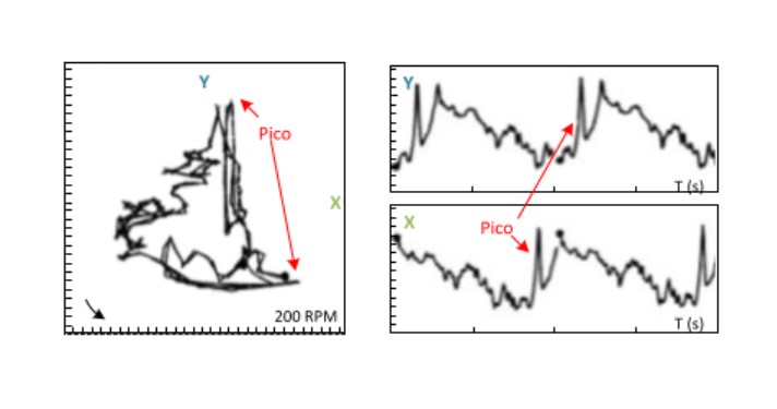
Remember that the positive peaks of the waveform represent the passage of the shaft next to the sensor and that, the mounting location of the sensors, is displayed on the orbit graph. The impulse of the phase sensor represents the same instant in all graphs. This combination of graphs makes it possible to correlate the information present in the orbit with the information of the waveforms.

17 – Measuring shaft center position with proximitors

The AC value of the signal measured with the proximitors gives us the vibrations of the shaft relative to the bearing. In the spectrum you can see numerous harmonics and inter-harmonics of the rotation speed at. In the spectrum you can see numerous harmonics and inter-harmonics of the rotation speed at. In the spectrum you can see numerous harmonics and inter-harmonics of the rotation speed at.

Below you can see a video measuring the position of the center of the shaft with proximitors.

Proximitors and full spectrum

Below you can see a video about measuring the full spectrum with proximitors.